SA380TX-L Applications
- Martyn Emmett (Unlicensed)
- Mark Beeson (Deactivated)
Digital acquisition
Digital event recording allows you to determine the present state of any relay (picked or dropped) and any change in state of any relay.
Front and Back Contacts
The TX-L allows you to monitor spare front (normally open) and spare back (normally closed) relay contacts.
Where back contacts are monitored the state of the relay will be the inverse of the state of the contacts.
To account for this discrepancy the TX-L gives you the option to configure a digital input as a front or back contact; the TX-L then automatically ensures the true state of the relay (picked or dropped) is captured.
State Changes
All digital inputs are continuously monitored for any change in state, whenever a change is detected the nature of the change is captured (UP to DN, or DN to UP) along with a timestamp accurate to within 10 mS.
Initial States
When the TX-L first boots, or restarts, it will capture the “initial state” of every digital input, this way you can see the present state of all monitored digital inputs at all times, even if no change in state has taken place on a particular channel.
Initial states are clearly indicated in the historical log, and are marked “UP” or “DN”. Initial states are not transmitted to the central server system.
Analogue acquisition
Acquire-on-Change
All analogue input channels are continuously logged using a process known as “Acquire-on-change”.
A sample is acquired when the measured value changes by more than a certain amount.
If there is no change, there is no sample acquired.
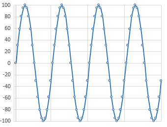
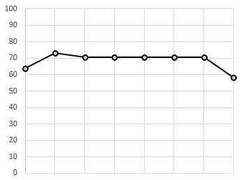
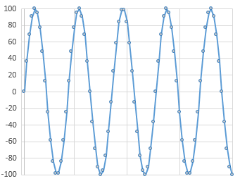
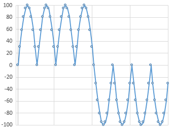
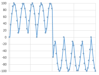
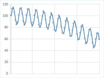
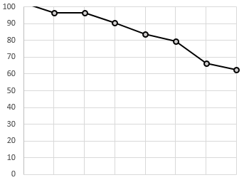
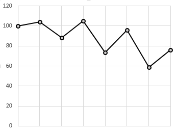
Consider the following waveform. The acquired samples are shown as dots.
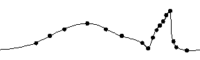
The waveform first changes at a fairly leisurely pace, then there is a spike. Each time the input changes significantly, a sample is acquired. It can be seen that more data points are acquired around the spike.
Acquire-on-change is an excellent match for many railway applications. Where there are long periods without much change, very little data is acquired. Where there is more detail in the waveform, more points are acquired.
After the data has been acquired it is possible to go back and just “join the dots” and we have an accurate representation of the entire waveform, with the minimum amount of data logged and transmitted.
Two methods of Acquire-on-Change are supported.
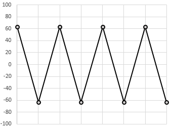
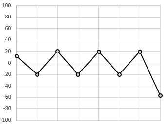
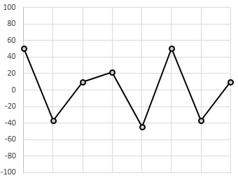
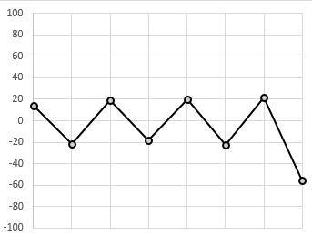
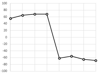
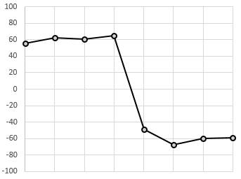
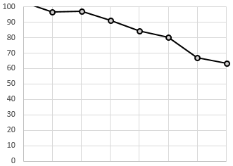
Absolute:
In absolute mode, a fresh sample is acquired each time the raw input signal changes by a fixed constant value, for example 5 mA.
E.g. If the last sample was acquired at 50 mA, the next sample will be acquired at +/- 5 mA, which is either 55 mA, or 45 mA. An absolute change of 5 mA is required to trigger the next acquisition.
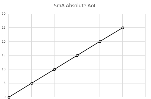
The chart above shows how samples would be acquired along a straight line slope.
Absolute acquisition is a good fit where the minimum and maximum range of the input signal are well known and an even level of detail is required at all ranges.
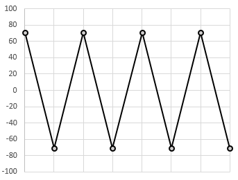
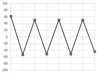
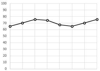
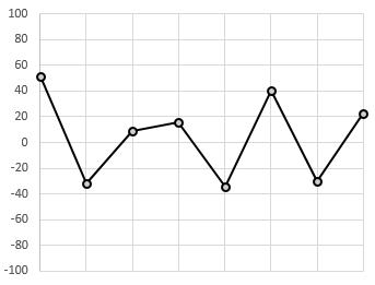
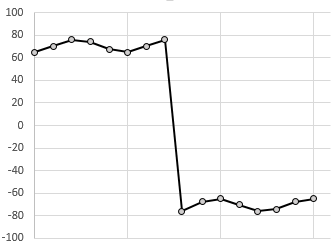
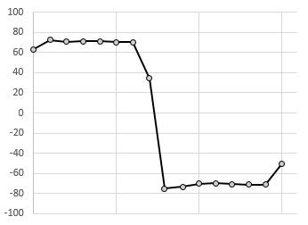
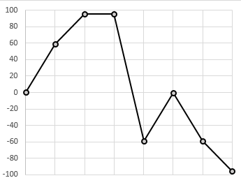
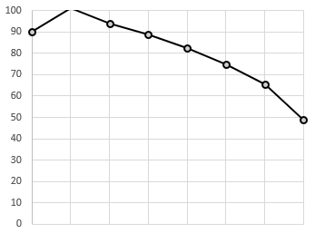
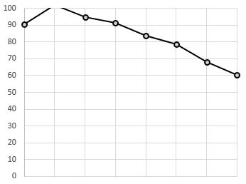
Relative:
In relative mode, a fresh sample is acquired each time the raw input signal changes by a defined percentage since the previous acquisition. It is defined in percent, for example 5%.
E.g. If the last sample was acquired at 50 mA, the next sample will be acquired at +/- 5% of 50 mA, which is either 52.5 mA, or 47.5 mA. A relative change of 5% is required to trigger the next acquisition.
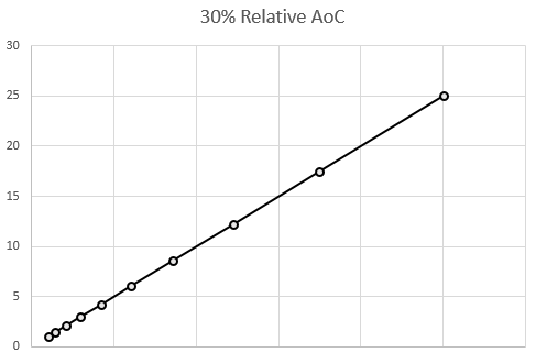
The chart above shows how samples would be acquired along a straight line slope.
Relative acquisition is a good fit where the minimum and maximum range of the input signal are not well known and where increased resolution is desired for small signals, at the expense of decreased resolution of large signals.
Example Applications for Acquire on Change:
- Rail Temperature Monitoring
- Track Circuit Monitoring
- Overhead Line Force and Displacement Monitoring
- Insulation Resistance Monitoring
- Power Consumption Monitoring
Triggered Capture
In addition to Acquire-on-Change you may also capture analogue data using a method known as “Triggered Capture”.
Triggered Captures are the method of choice when you want to record intermittent railway events at maximum resolution.
A triggered capture will begin recording when a “start trigger event” is detected.
Analogue data on the selected channel will then be recorded at maximum resolution until a “stop trigger event” is detected.
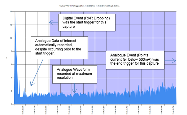
A trigger event can be fired by a change in state of a digital input, or by an analogue input transitioning through a pre-determined threshold level.
Sometimes analogue data of interest can lie just outside the time-window defined by the start and end trigger events. To combat this, the TX-L will automatically include analogue data of interest up to 1 second either side of the start and end trigger events in the final triggered capture waveform.
Where you are monitoring assets that may move in two directions, you may also assign a direction (Normal to Reverse or Reverse to Normal) to a triggered capture. In the event that the logger cannot determine direction, the direction will be labelled invalid.
Example Applications:
- Point Condition Monitoring
- Powered Mechanical Signal Monitoring
- Level Crossing Barrier Monitoring
- Boom / Wig-Wag Lamp Monitoring
Input Scaling
- The SA380TX-L is designed to accept 4-20mA current transducers
- The 4-20mA signal must be scaled into the engineering units of the metric being measured.
- This requires setting the engineering units, (e.g. mA, N, oC, V etc).
- This requires selecting a scaling method and defining scaling parameters
Three methods of scaling are supported:
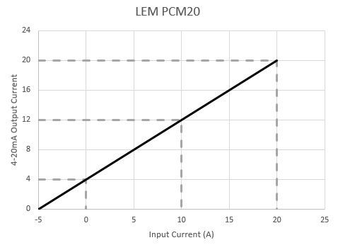
Scaling Name Description Example(s) Linear By far the most common method of scaling. Most 4-20mA sensors specify the output at 4mA and at 20mA. The sensor output is considered linear between these two points This is the typical usable range of the sensor, however many sensors continue to drive outputs below 4mA and beyond 20mA when excited beyond their normal working range. LEM PCM20 (0 to +20 Amp Sensor)
Value at 4mA = 0 A
Value at 20mA = 20 A
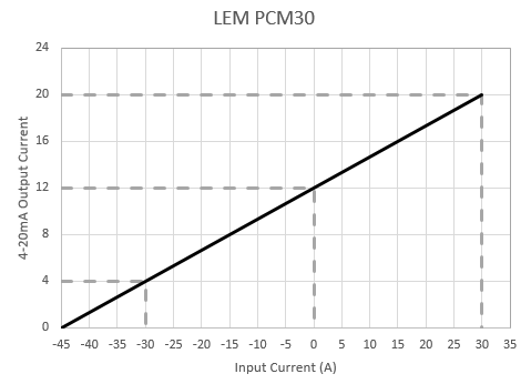
 LEM PCM30 (+/-30 Amp Sensor)
Value at 4mA = -30 A
Value at 20mA = 30 A
Quadratic Rarely, the output of a 4-20mA sensor may be non-linear. This may be due to the requirement to measure an exponentially varying signal, or a limitation of the sensor technology. In such scenarios it is possible to "fit" the sensor response to a 4-20mA curve using a polynomial expression in the form: y = ax2 + bx + c where 'x' is the 4-20 mA input signal, and 'y' is the desired output parameter. Suitable values for a, b and c should be provided by the sensor supplier. Findlay Irvine 407 (-20 to +60 oC Sensor)
a = -0.443
b = +16.063
c = -89.557
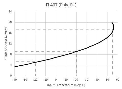 The curve fit may be acceptable for some applications, however an Inverse Polynomial fit gives less error for this sensor.
Inverse Quadratic Rarely, the output of a 4-20mA sensor may be non-linear. This may be due to the requirement to measure an exponentially varying signal, or a limitation of the sensor technology. In such scenarios it is possible to "fit" the sensor response to a 4-20mA curve using a polynomial expression in the form: y = (a / x2)+ (b / x) + c where 'x' is the 4-20 mA input signal, and 'y' is the desired output parameter. Suitable values for a, b and c should be provided by the sensor supplier. Findlay Irvine 407 (-20 to +60 oC Sensor)
a = +722.7
b = -768.6
c = 96.419
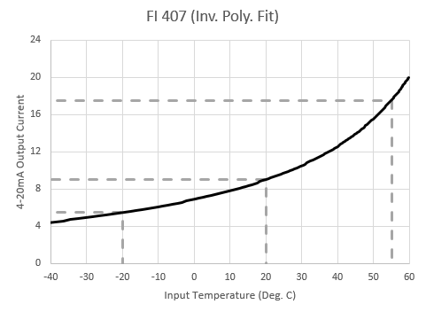 The inverse polynomial curve fit is good for this sensor, producing less than 1 oC of error at any point of the response curve.
Filtering
- The SA380TX-L will nominally sample analogue inputs at 1,000 samples per second.
- The sample rate may be reduced to increase the maximum length in time of triggered captures if desired.
- There is no hardware anti-alias filter. Any input signal with frequency components greater than half the sample rate will cause aliasing of data.
- Input data is first filtered using one of several filtering algorithms described below.
- After filtering, the data is decimated by a factor of 10, to a lower sample rate.
The following data rates are supported:
| Input Rate | Output Rate | Maximum Capture Length |
|---|---|---|
| 1000 Hz | 100 Hz | 7.5 sec. + 1 sec. each pre/post trigger |
| 625 Hz | 62.5 Hz | 13.2 sec. + 1 sec. each pre/post trigger |
| 500 Hz | 50 Hz | 17 sec. + 1 sec. each pre/post trigger |
| 333 Hz | 33.3 Hz | 26.5 sec. + 1 sec. each pre/post trigger |
| 250 Hz | 25 Hz | 36 sec. + 1 sec. each pre/post trigger |
- Data is fed at the output rate to the "triggered capture" and "acquire on change" data acquisition processes.
- Careful consideration should be given to the selection of filter type.
The table below explains each filter setting and demonstrates its action upon incoming data.
- The ideal filters for common input waveform types is highlighted in Green.
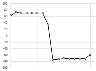
- Filters that will cause highly erroneous data output are highlighted in Red.
| Input Signal | Raw Signal (1 kHz) | Arithmetic Mean | AC RMS | DC RMS | AC RMS with Low Pass Filter | DC RMS with Low Pass Filter | Low Pass Filter | Pass Through |
|---|---|---|---|---|---|---|---|---|
| Behaviour | Calculates a pure average of a 10 input sample block. | Calculates the true RMS value of a 10 sample block | Calculates the true RMS value of a 10 sample block. The algorithm preserves the "sign" of the input signal, hence negative values can still be reported. | Calculates the true RMS value of a 10 sample block, and then implements a 20 dB per decade low-pass-filter with a cut-off frequency of 0.4 x the output sample rate. | Calculates the true RMS value of a 10 sample block. The algorithm preserves the "sign" of the input signal, hence negative values can still be reported. Also implements a 20 dB per decade low-pass-filter with a cut-off frequency of 0.4 x the output sample rate. | Implements a 20 dB per decade low-pass-filter with a cut-off frequency of 0.4 x the output sample rate. | Simple decimation. 9 out of 10 samples are dropped, every 10th sample gets through. Does not apply any scaling | |
| Useful for | Linear sensors, such as force or temperature sensors | AC motors and systems fed from 50 Hz supplies | DC Motors and systems fed from full-wave rectified 50 Hz supplies. | AC motors and systems fed from 60 Hz supplies, or where additional smoothing is desirable. | DC Motors and systems fed from full-wave rectified 60 Hz supplies, or where additional smoothing is desirable. | Linear sensors where the simple average filter produces noisy output | Diagnostic and Experimentation. Not typically used in every-day installations. | |
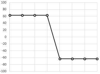
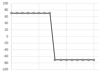
| 50 Hz AC |
|
|
|
|
|
|
|
|
| 60 Hz AC |
|
|
|
|
|
|
|
|
| 50 Hz DC |
|
|
|
|
|
|
|
|
| 60 Hz DC |
|
|
|
|
|
|
|
|
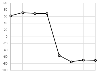
| Wandering Signal |
|
|
|
|
|
|
|
|

EbiTrack® Digital Transmitter / Receiver Acquisition
Each EbiTrack unit reports a mixture of analogue data, digital data, and error state information, roughly once per second. EbiTrack 200, 300 and 400 digital receivers are supported, as are EbiTrack 400 digital transmitters.
Digital
Digital data is captured in the same manner as regular digital inputs
Analogue
Most analogue data is captured by the TX-L using standard "Acquire-on-Change" rules in exactly the same manner as regular analogue inputs.
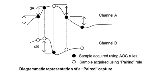
Paired Analogue
The following analogue data is also captured by the TX-L following “Acquire-on-change” rules, however, when data is captured on one analogue channel, data is also simultaneously captured on a paired “sister” channel (see below).
Data capture continues for 5 seconds after the last significant change was detected. This is in order to comply with Network Rail data acquisitions specifications in the UK.
- Lower Sideband Current, paired with Upper Sideband Current (EbiTrack 200/300 Rx Only)
- Relay Output Voltage, paired with Relay Output Current (Except EbiTrack 400 Tx)
Error Data
Whenever a receiver reports error data, the following information is recorded.
- Error Code
- Serial Number
- Mod State
- Frequency Code
- Key Number
- Autoset Key Number (Except EbiTrack 400 Tx)
- Current Threshold (Except EbiTrack 400 Tx)
Some of this data is sent as a "text" event.
Channel Summary
The table below summarises the data acquired from each EbiTrack Model.
| EbiTrack Channel Name | Channel Meaning | Type | EbiTrack 200 / 300 Rx | EbiTrack 400 Rx | EbiTrack 400 Tx | Notes |
|---|---|---|---|---|---|---|
| TEMP | Temperature | Ana | Y | Y | Y | |
| VPSU | PSU Voltage | Ana | Y | Y | Y | |
| SERN | Serial Number | Text | Y | Y | Y | |
| MODS | Mod State | Text | Y | Y | Y | |
| FREQ | Frequency | Text | Y | Y | N | |
| KYSN | Key Serial Number | Text | Y | Y | Y | |
| EADD | Last Error Code | Ana | Y | Y | Y | |
| ASSN | Autoset Key Number | Ana | Y | Y | Y | |
| ITHR | Threshold Current | Ana | Y | Y | N | |
| VOUT | Output Voltage | Ana | Y | Y | N | Paired with Output Current |
| IOUT | Output Current | Ana | Y | Y | N | Paired with Output Voltage |
| IUSB | Upper SIde-band Current | Ana | Y | N | N | Paired with Lower Side-band Current |
| ILSB | Lower Side-band Current | Ana | Y | N | N | Paired with Upper Side-band Current |
| IAVE | Average Current | Ana | Y | Y | N | |
| IERR | Error State | Dig | Y | Y | Y | |
| VOPD | Output Drive Voltage | Ana | N | N | Y | |
| POPD | Output Drive Power | Ana | N | N | Y | |
| TFET | Drive FET Temperature | Ana | N | N | Y | |
| TTRN | Drive Transformer Temperature | Ana | N | N | Y | |
| OMSN | Output Module Serial No. | Text | N | N | Y | |
| OMMS | Output Module Mod State | Text | N | N | Y | |
| ITOT | Total Input Current | Ana | N | Y | N | |
| SBRT | Side-band Current Ratio | Ana | Y | N | N |
Storage and transmission
Storage
All data recorded by the TX-L is stored on a non-volatile disk internal to the logger. The TX-L guarantees to store all captured data for a minimum period of 31 days.
When the disk becomes full, old data is written over and permanently erased, however it is always the oldest data that is deleted first.
The SA380TX-L does not feature duplicated data storage and as such cannot be classed as a “Digital Event Recorder” as per Network Rail standards. This means that the TX-L is unsuitable for use as a judicial event recorder on Network Rail infrastructure.
Transmission
The TX-L is designed to be used in conjunction with a central data storage server and offers two mediums that allow data recorded trackside to be transmitted to a central repository.
At present two data storage server systems support the TX-L logger:
- The Network Rail Intelligent Infrastructure “Wonderware” server. This is presently preferred by Network Rail for all Intelligent Infrastructure data loggers.
- The MPEC “Centrix” Server. For other organisations or for NR infrastructure not within scope of the NR II program please contact MPEC for more information about Centrix.
- www.centrix.org
GPRS
In locations where no physical telecoms infrastructure exists then data can be sent over-air using the in-built GSM modem. The modem uses GPRS to transmit the data.
Ethernet
Where physical telecoms infrastructure is supported higher data rates and better reliability can be achieved by connecting the logger over Ethernet. The units’ 24v DC 2W auxiliary power supply is designed to power an external modem or router to allow the TX-L to connect to a wide array of telecoms infrastructure via Ethernet.
Contact MPEC or your telecoms engineer to discuss an Ethernet installation.